Image classification is used on overhead imagery to detect specific objects such as planes, cars and buildings. Creating and training effective deep learning image classification models is dependent on the proper tuning of model hyper-parameters, along with appropriate image preprocessing and standardization.
Big Questions
What is the difference in model performance between models trained on 16-bit images and models trained on images converted to 8-bit?
How should images pixel values be standardized?
Should standardization be based on only a collection of local or global pixel intensities?
16 bit vs 8 bit Imagery
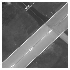
Within an image, digital information is stored in pixels as intensities or tones. An 8-bit image can hold 256 different intensities within a single image channel; a standard color image has 3 channels - red, green and blue (RGB). Thus, each pixel in a standard RGB image consumes 24 bits of information. In all, RGB 8 bit images can hold up to 16.7 Million different values. 16 Bit images, on the other hand can hold 65,536 pixel intensities in a single channel, resulting in 28 Billion possible values. This is a significant difference, several orders of magnitude larger, and has implications in how this data is processed.
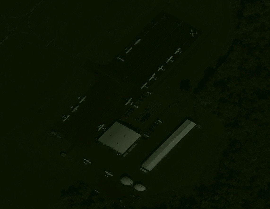
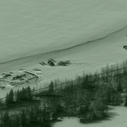
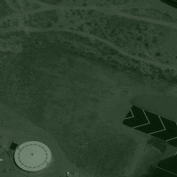
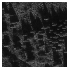
Figure 1: On the left is an example 16 bit satelite image on the right is an image that was 16 bit, but has been converted to 8 bit.
Challenges
In addition to being 16-bit, satellite imagery is huge, generally on the order of tens of thousands of pixels in width and height. All images used in this blogpost are derived from the Rareplanes Dataset which includes panchromatic (single channel) imagery of different airports with over ten thousand labeled planes. To train an image classification model, we needed to "chip" the full images into smaller tiles that could then be converted and standardized to be fed into a model.
Using the metadata associated with each satellite image, we located the centroid of each labeled plane within each image. We then used those coordinates to create 512 x 512 chips around each plane using gdal to create our "positive" chips. "Negative" chip generation conversely used those coordinates to exclude planes entirely and only chip non-plane areas. In generating the negative chips, it is important to include as wide a variety of non-plane data as possible, to help reduce the number of false positive detections of the model. We generated one thousand 512 x 512 negative chips per positive chip.
We trained an airplane detector on the Rareplanes dataset using five different image standardization methods, two using 16-bit imagery, and three using 16-bit converted to 8-bit imagery. The following cards display the normalization methods used for each case.
Cases
Hover over the image below to see normalization methods:
We trained an airplane detector on the Rareplanes dataset using five different image standardization methods, two using 16-bit imagery, and three using 16-bit converted to 8-bit imagery. The following cards display the normalization methods used for each case.
Training
The model utilized a ResNet50 Architecture modified to accept single color imagery as input. The dataset included 187 total satellite images which were used to generate 10901 positive chips and 180000 negative chips, all of 256*256 dimensions. Each case was then trained from scratch for 60 iterations with a 70/30 train/val random split created for robust training. Every case has the same train and val set. However, different data augmentation functions such as horizontal and vertical shifts, horizontal and vertical flips, random rotations, blurs, and crops were randomly applied throughout.
Validation
In this step we performed an Initial evaluation of the model on validation data. This analysis determined the appropriate threshold a predicted probability must exceed in order to be classified as a positive. The goal was to minimize the number of false positive and false negative predictions. We use the metrics below to inform which thresholds were selected for each model.
True Positives
False Positives
True Negatives
False Negatives
Accuracy: True Positives plus True Negatives, divided by the Total Chips
True Positive Rate: Percent of True Positives given a threshold.
False Positive Rate: Percent of False Positives given the threshold. This was one of the most important metrics in determining the appropriate threshold. This often was comes at the expense of FN.
False Negative Rate: Percent of false negative given the threshold.
"Augmented" False Positives: This curated metric took the the number of FPs produced from the validation set and linearly scaled that number to represent how many FPs we would expect if we were to insert a full image worth of chips into the model. Given every image is on average 65,000 x 65,000 pixels, with batch sizes of 50 or more images, there would be 85 times the size of the validation set worth of chips being processed through the model on average. Therefore, the Augmented FPs scales the number of FPs by a factor of 85.
In all five cases, the central deciding factor in threshold selection was the Augmented FP. At lower thresholds accuracy, TP rate and FN rate all do well. At thresholds close to 0, nearly all probabilities are classified as positive. Therefore the number of FN also decreases. Alternatively, FPs increase drastically by lowering the threshold. Therefore, thresholds were set at the lowest probability where the Augmented FP was less than 100. This both satisfies a low expected FP count while optimizing accuracy, TPR and FNR. One hundred is a number that can easily be modified by a client based on individual tolerance, but for the purposes of these experiments we used it.
1. Test on 512*512 chips and return one classification that details whether ANY plane exists in chip or no planes exist at all. (Does not count number of planes)
2. Test on full size satellite image or 15000*15000 chips of that image (whichever is smaller). Counts how many planes exist and returns visualization with plane locations highlighted.
Results Table:
Test Method 1
Test Method 2
Case
Threshold
TP
FP
TN
FN
Precision
Recall
F1 Score
TP
FP
FN
Precision
Recall
F1 Score
1
0.55
2086
2
61512
1721
0.999
0.547
0.707
2697
1635
8204
0.623
0.247
0.354
2
0.60
2115
3
61511
1692
0.9986
0.556
0.714
2652
1319
8294
0.665
0.243
0.356
3
0.65
2059
1
61513
1748
0.9995
0.541
0.702
1916
829
8985
0.698
0.176
0.297
4*
0.60
1913
9
61505
1894
0.9953
0.503
0.668
2023
1126
8878
0.642
0.186
0.288
5
0.70
1658
2
61512
2149
0.9988
0.436
0.607
1242
1046
9659
0.543
0.114
0.188
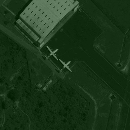
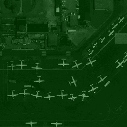
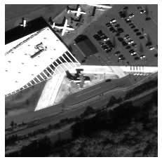
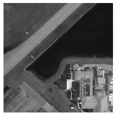
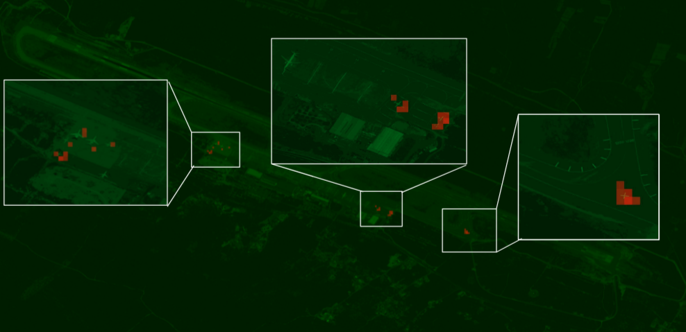
Test Method 2 Example Result Image:
This figure is an example output for test method 2. Detections over the estaablished threshold for each case display as read heatmap like detections. This image was normalized using Case 1 techniques with a detection threshold of 0.55.